Range-Doppler Estimation
In this lesson, you will learn about the basics of range and velocity estimation using doppler and Fourier transform techniques. Before you get started, let's have a look at three primary dimensions of measurement for radar resolution.
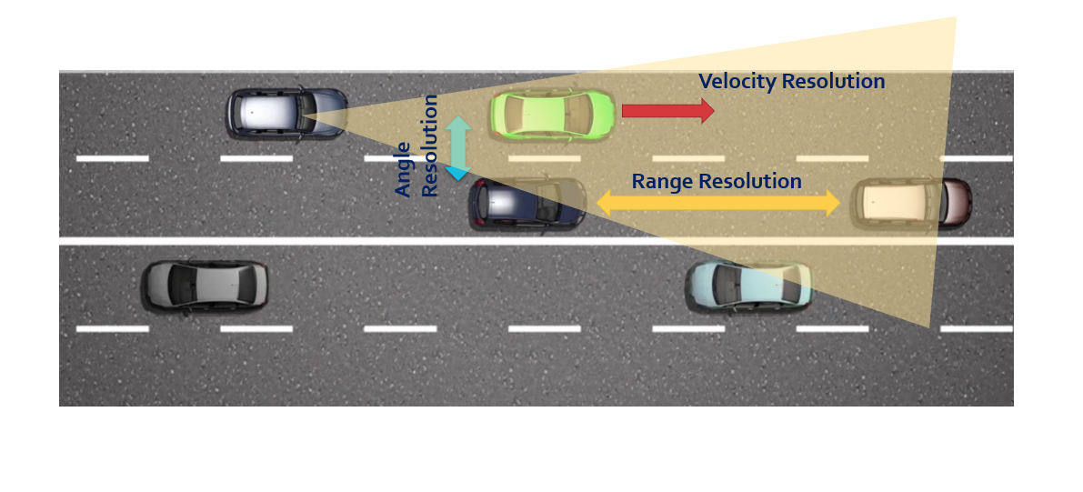
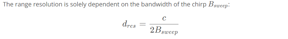
Range Resolution: It is the capability of the radar to distinguish between two targets that are very close to each other in range. If a radar has range resolution of 4 meters then it cannot separate on range basis a pedestrian standing 1 m away from the car. Higher bandwidth would allow smaller range resolution. This will help radar distinguish between close range targets.
Velocity Resolution: If two targets have the same range they can still be resolved if they are traveling at different velocities. The velocity resolution is dependent on the number of chirps. As discussed for our case we selected to send 128 chirps. A higher number of chirps increases the velocity resolution, but it also takes longer to process the signal.
Angle Resolution: Radar is capable of separating two targets spatially. If two targets are at similar range travelling at same velocities, then they can still be resolved based on their angle in radar coordinate system. Angle resolution depends on different parameters depending on the angle estimation technique used.
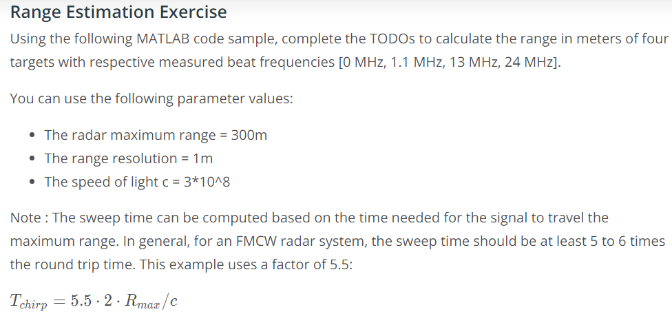
Range Estimation
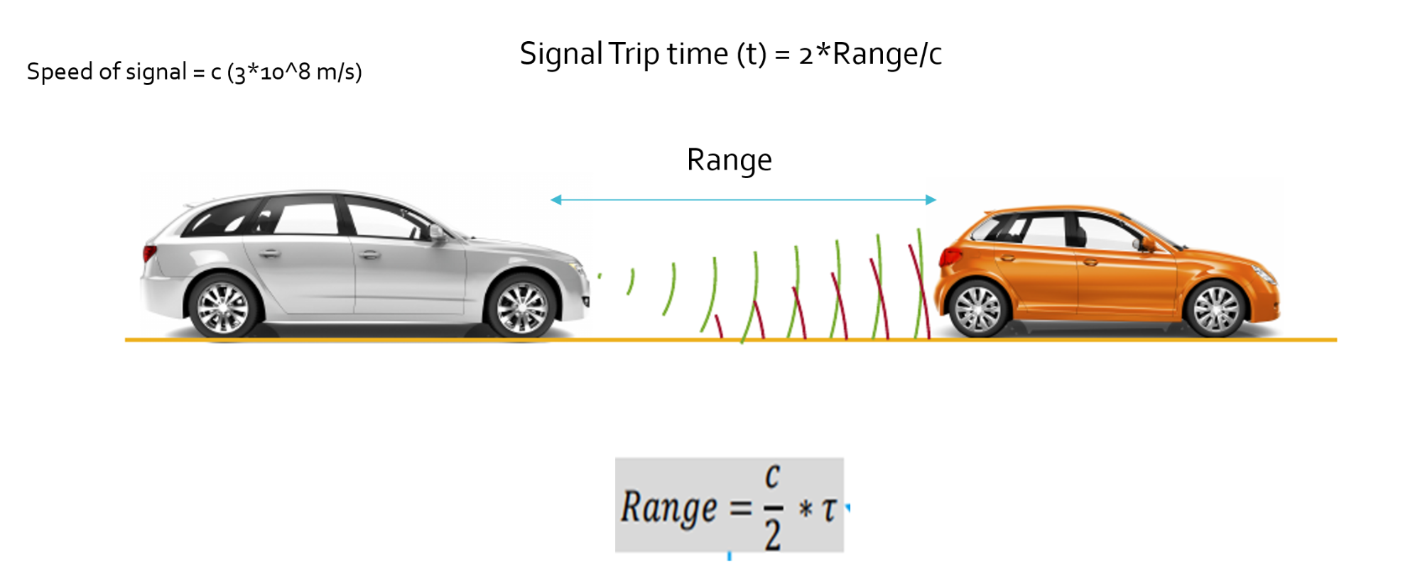
Radar determines the range of the target by measuring the trip time of the electromagnetic signal it radiates. It is known that EM wave travels at a known speed (300,000,000 m/s), so to determine the range the radar needs to calculate the trip time. How?
Answer : By measuring the shift in the frequency.
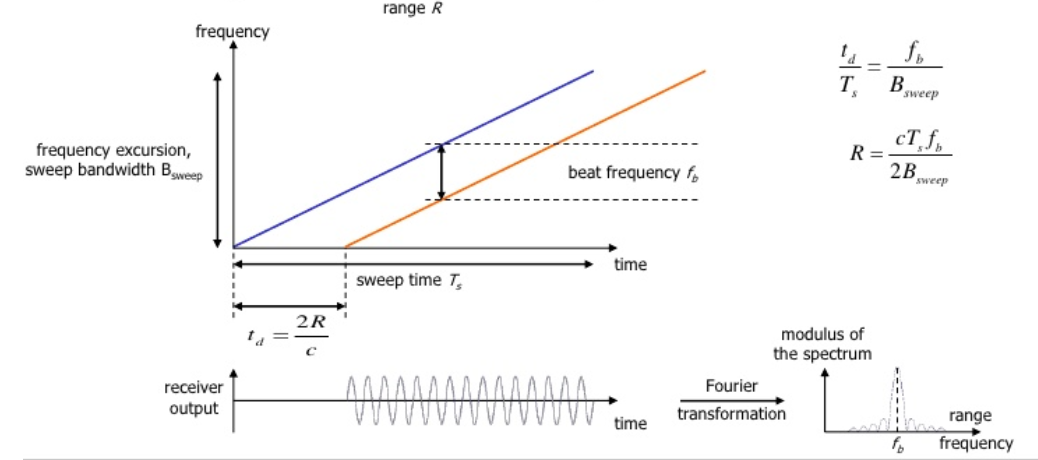
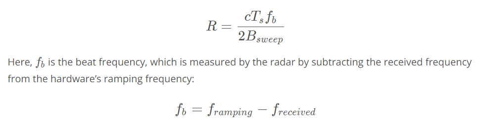
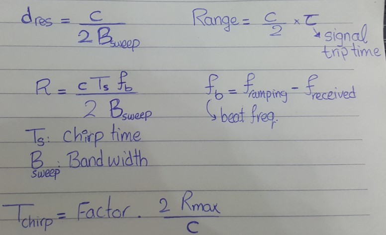
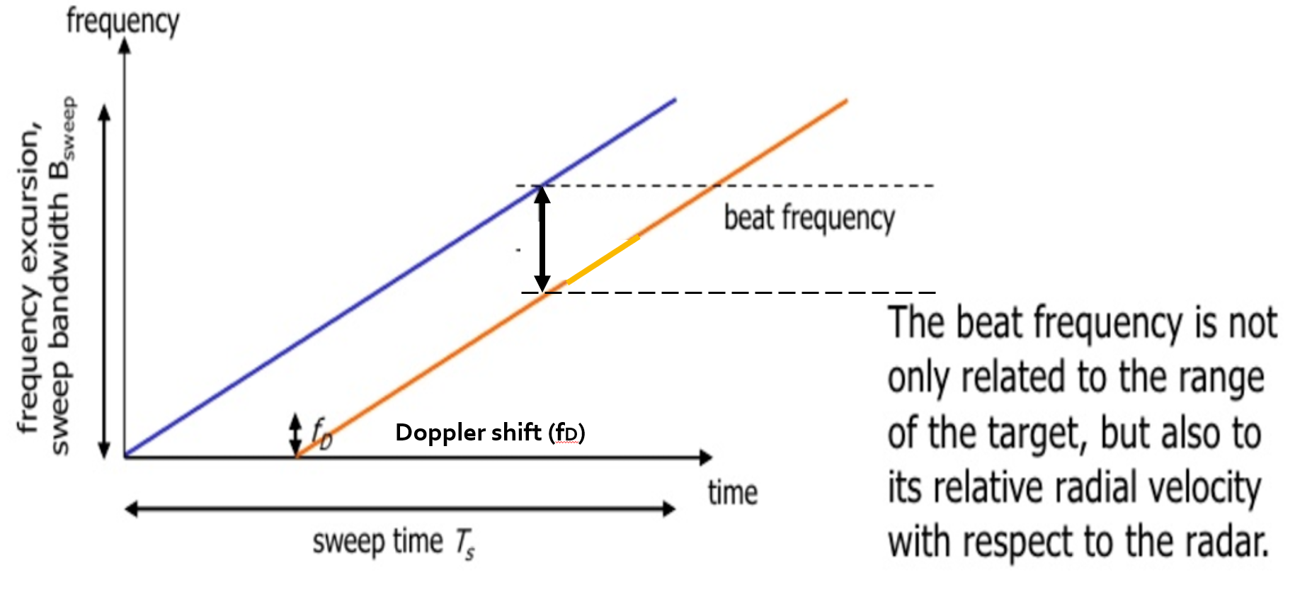
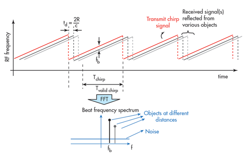
The FMCW waveform has the characteristic that the frequency varies linearly with time. If radar can determine the delta between the received frequency and hardware’s continuously ramping frequency then it can calculate the trip time and hence the range. We further divide Range estimate by 2, since the frequency delta corresponds to two way trip.
It is important to understand that if a target is stationary then a transmitted frequency and received frequency are the same. But, the ramping frequency within the hardware is continuously changing with time. So, when we take the delta (beat frequency) between the received and ramping frequency we get the trip time.
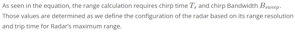
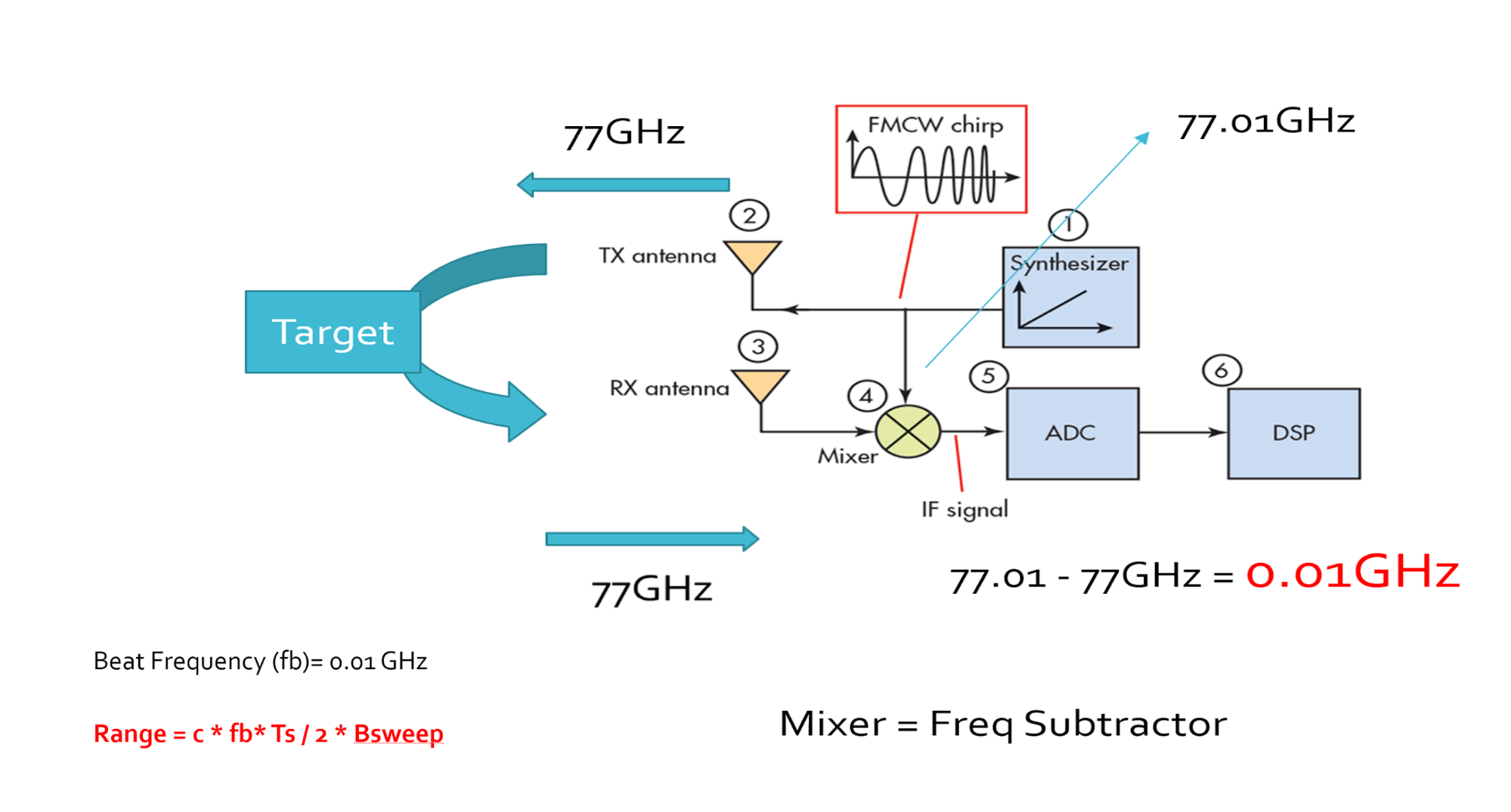
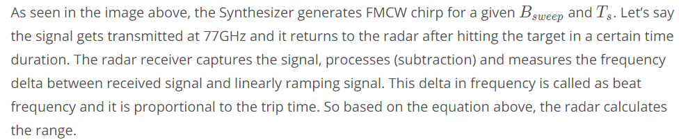
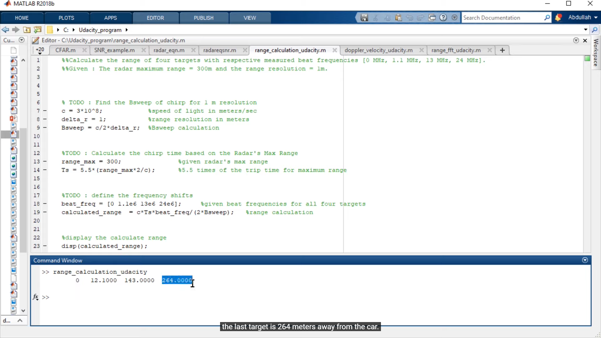
System Level Range Calculation
Note : The sweep time can be computed based on the time needed for the signal to travel the maximum range. In general, for an FMCW radar system, the sweep time should be at least 5 to 6 times the round trip time
Summary of Rules
Doppler Estimation
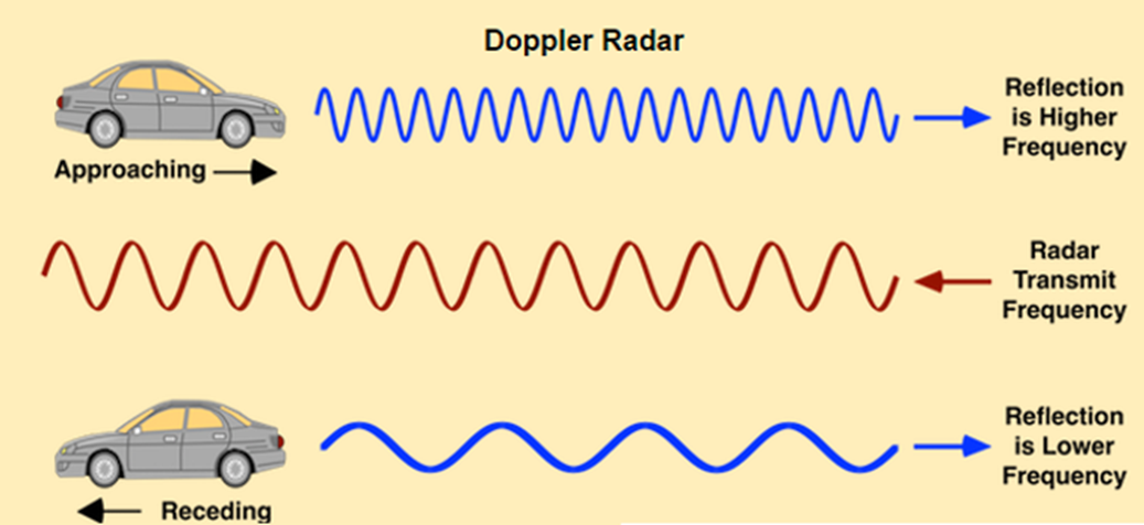
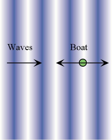
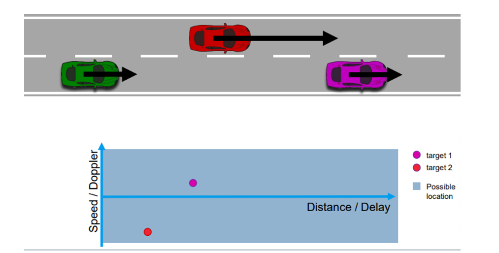
The velocity estimation for radar is based on an age old phenomenon called the doppler effect. As per doppler theory an approaching target will shift an emitted and reflected frequency higher, whereas a receding target will shift the both frequencies to be lower than the transmitted frequency.
Doppler effect is the change in frequency of a wave reflected off a moving target. If we have one moving object in the scene, when the target is moving, the received signal that is reflected back to the radar might arrive earlier than expected if the target is moving towards the radar. That is because the current wave is reflected from a position which is closer to the sensor, and similarly the signal might arrive with a delay if the target is moving away. This is also translated as a higher or lower frequency.
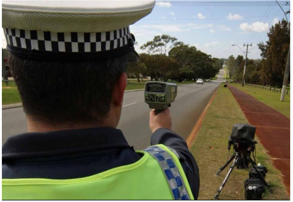
The same principle is used in the radar guns to catch the speed violators, or even in sports to measure the speed of a ball.
There will be a shift in the received signal frequency due to the doppler effect of the target’s velocity. The doppler shift is directly proportional to the velocity of the target as shown below.
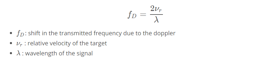
By measuring the shift in the frequency due to doppler, radar can determine the velocity. The receding target will have a negative velocity due to the frequency dropping lower, whereas the approaching target will have positive velocity as the frequency shifts higher.
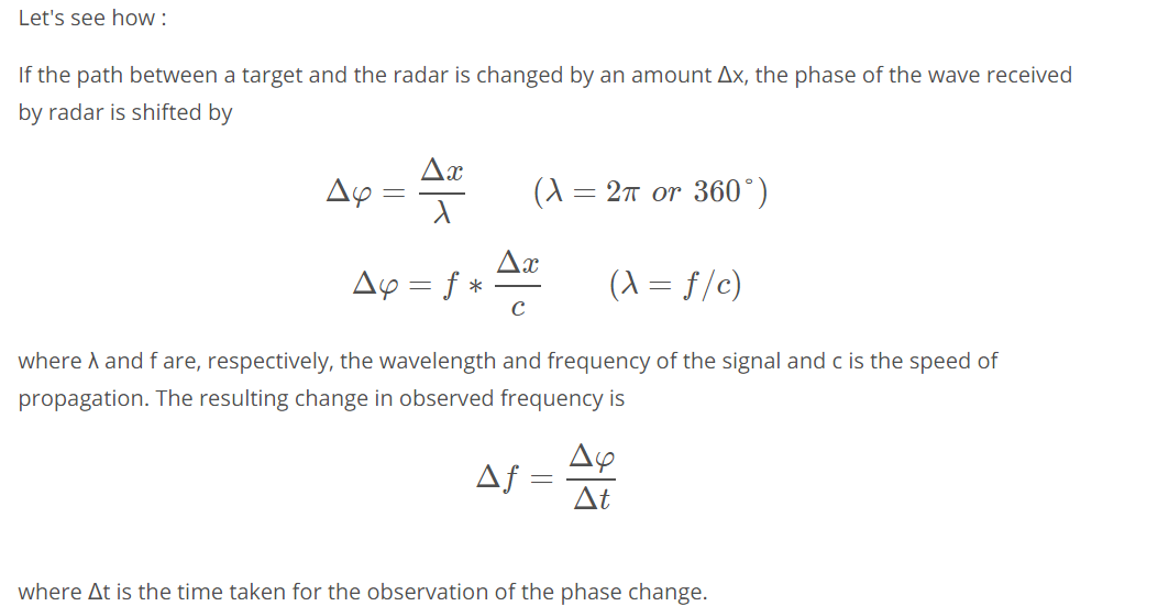
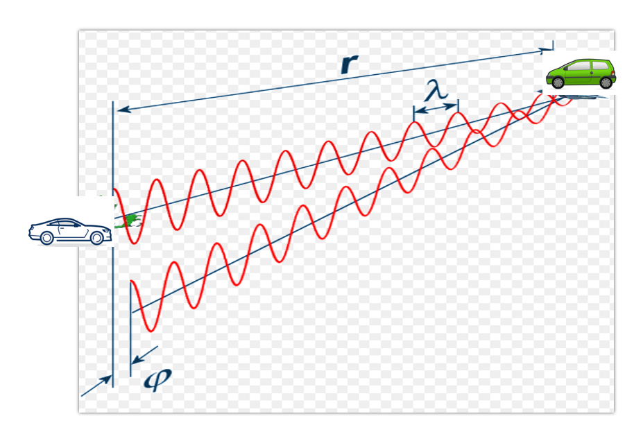
DOPPLER PHASE SHIFT
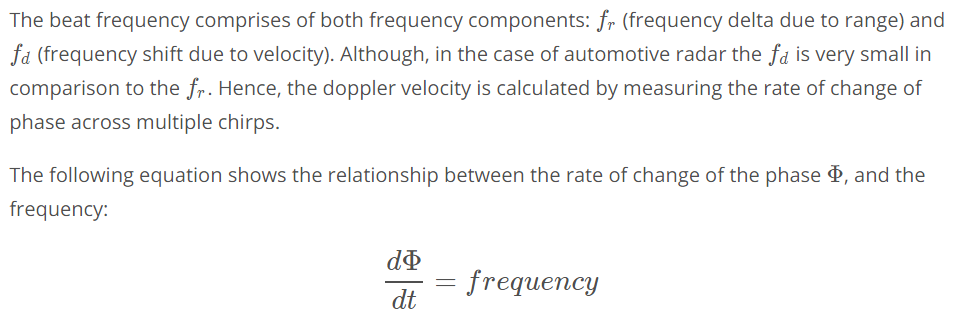
Keeping that in consideration, we calculate the doppler frequency by measuring the rate of change of phase. The phase change occurs due to small displacement of a moving target for every chirp duration. Since, each chirp duration is generally in microseconds, it results in small displacement in mm (millimetres). These small displacements for every chirp leads to change in phase. Using this rate of change of phase we can determine the doppler frequency.
Fast Fourier Transform (FFT)
So far we discussed the theory of range and doppler estimation along with the equations to calculate them. But, for a radar to efficiently process these measurements digitally, the signal needs to be converted from analog to digital domain and further from time domain to frequency domain.
ADC (Analog Digital Converter) converts the analog signal into digital. But, post ADC the Fast Fourier Transform is used to convert the signal from time domain to frequency domain. Conversion to frequency domain is important to do the spectral analysis of the signal and determine the shifts in frequency due to range and doppler.
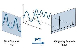
The traveling signal is in time domain. Time domain signal comprises of multiple frequency components as shown in the image above. In order to separate out all frequency components the FFT technique is used.
For the purpose of this course we don’t have to get into mathematical details of FFT. But, it is important to understand the use of FFT in radar’s digital signal processing. It gives the frequency response of the return signal with each peak in frequency spectrum representing the detected target’s characteristics.
 https://www.youtube.com/watch?v=t_NMmqTRPIY&feature=youtu.be
As seen in the image below, the Range FFTs are run for every sample on each chirp. Since each chirp is sampled N times, it will generate a range FFT block of N * (Number of chirps). These FFT blocks are also called FFT bins.
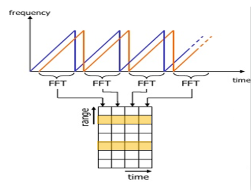
Each chirp is sampled N times, and for each sample it produces a range bin. The process is repeated for every single chirp. Hence creating a FFT block of N*(Number of chirps).
Each bin in every column of block represents increasing range value, so that the end of last bin represents the maximum range of a radar.
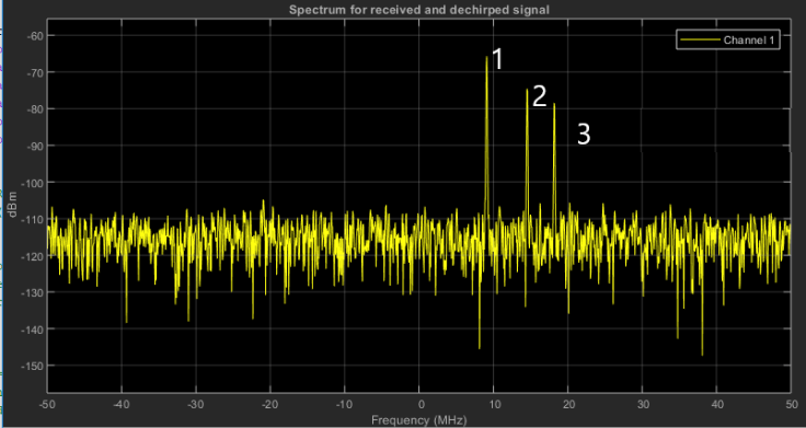
Above is the output of the 1st stage FFT (i.e Range FFT). The three peaks in the frequency domain corresponds to the beat frequencies of three different cars located at 150, 240 and 300 m range from the ego vehicle.
The 2D FFT
Once the range bins are determined by running range FFT across all the chirps, a second FFT is implemented along the second dimension to determine the doppler frequency shift. As discussed, the doppler is estimated by processing the rate of change of phase across multiple chirps. Hence, the doppler FFT is implemented after all the chirps in the segment are sent and range FFTs are run on them.
The output of the first FFT gives the beat frequency, amplitude, and phase for each target. This phase varies as we move from one chirp to another (one bin to another on each row) due to the target’s small displacements. Once the second FFT is implemented it determines the rate of change of phase, which is nothing but the doppler frequency shift.
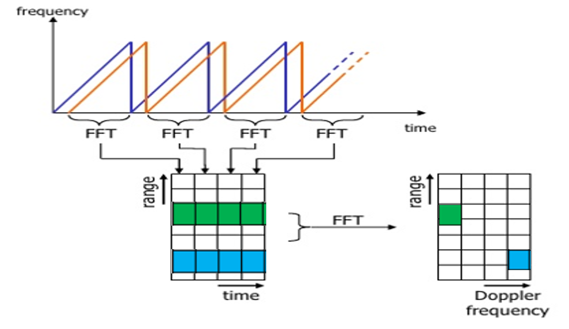
After running 2nd FFT across the rows of FFT block we get the doppler FFT. The complete implementation is called 2D FFT. After 2D FFT each bin in every column of block represents increasing range value and each bin in the row corresponds to a velocity value.
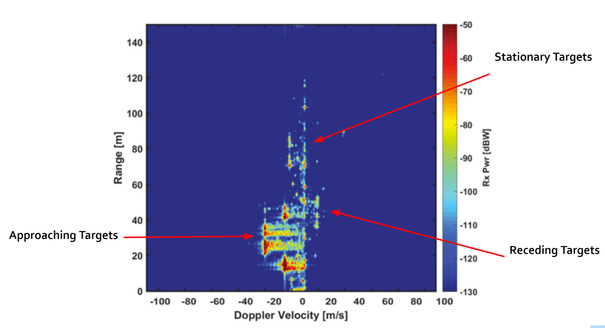
The output of Range Doppler response represents an image with Range on one axis and Doppler on the other. This image is called as Range Doppler Map (RDM). These maps are often used as user interface to understand the perception of the targets.
For more information about the 2D FFT